Evaluation Tutorial

(It is recommended that readers take a look at our paper to understand the idea underlying this tutorial.)

Just try it!

Jupyter notebook released!

A new jupyter notebook for those who just want result can be found here.

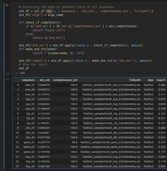
Fig 1. Output of the Jupyter script.

The script will take care of the intricacies in evaluating odometry output with external ground truth. If you are interested in learning more about these intricacies, please read through the tutorial below!

MATLAB

This is the original evaluation script for NTU VIRAL.

You can download an example of how to calculate the absolute trajectory error (ATE) of the position estimate from the github repo. Fig. 2 gives an overview of the package's content.

The code was written and verified on MATLAB 2020a. Upon downloading, simply run the script evaluate_all.m and the ATE of each trial will be calculated, assembled and printed out on the Command Window. Data plots and numerical results are also saved into the appropriate directories.

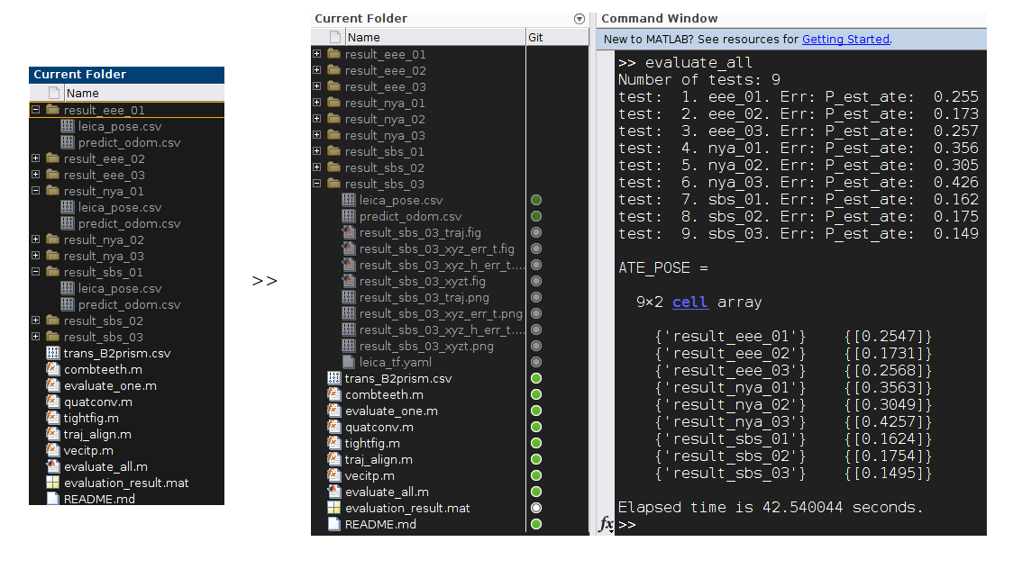
Fig 2. The content of the evaluation package, and outputs after running the evaluation script

The package contains multiple MATLAB scripts and several log files of the ouput of our SLAM method. Specifically the logs are created by calling the following commands before launching the SLAM method in a ubuntu terminal.

timeout $LOG_DUR rostopic echo -p --nostr --noarr /viral_slam/pred_odom > $OUTPUT_DIR/predict_odom.csv &
timeout $LOG_DUR rostopic echo -p --nostr --noarr /leica/pose/relative  > $OUTPUT_DIR/leica_pose.csv;

where $LOG_DUR is essentially be the duration of the bag file (some buffering time should be added) and $OUTPUT_DIR is the targeted output directory.

Below we will break down the main parts of the evaluation script, which would be useful if you seek to adopt this for evaluating your algorithm's output.

evaluate_all.m

Most commands in this script are self-expressive, we only take note at the following line in evaluate_all.m:

tests       = dir([this_dir 'result_*']);

The above command assumes that we prefix the folders containing the results with result_ for MATLAB to check their presence. Readers can change to another indicator as they like by changing the variable $OUTPUT_DIR above.

Looking into this script, readers can see that it simply checks out the folders starting with the same name and iteratively passes the folder name to evaluate_one.m to obtain the ATE estimate. Let us delve in to this script in the next part.

evaluate_one.m

Reading the data from logs

Most commands in this script are also self-explanatory, thus we will comment on important sections. First notice the following part

gndtr_pos_fn     = [exp_path 'leica_pose.csv'];
pose_est_fn      = [exp_path 'predict_odom.csv'];
trans_B2prism_fn = [exp_path '../trans_B2prism.csv'];


%% Read the gndtr data from logs

% Position groundtr
gndtr_pos_data = csvread(gndtr_pos_fn,  1, 0);

% First sample time used for offsetting all others
t0_ns = gndtr_pos_data(1, 1);

% pos groundtruthdata
t = (gndtr_pos_data(:, 1) - t0_ns)/1e9;
P = gndtr_pos_data(:, 4:6);

Thus, it is noted that we assume the groundtruth, estimate, and the prism's coordinates are logged in files of specific names as shown above. Also, we have assumed that the 1st column of the leica_pose.csv file is the timestamp, and column 4, 5, 6 are position estimate. These indices are in accordance with the log of a geometry_msgs::PoseStamped topic logged with the aforementioned rostopic commands.

Similarly we notice the next part

%% Read the viralslam estimate data from logs
% SLAM estimate
pose_est_data = csvread(pose_est_fn, 1, 0);
t_est = (pose_est_data(:, 1) - t0_ns)/1e9;
P_est =  pose_est_data(:, 4:6);
Q_est = (pose_est_data(:, [10, 7:9]));
V_est =  pose_est_data(:, 11:13);

Obviously, the first 5 commands extract the position, quaternion and velocity estimates from the log file predict_odom.csv. The indices are in accordance with the log of a nav_msgs::Odometry topic. This is our preferred message type since it already has definition for position, quaternion and velocity. If the user chooses a different message type for their output, the indices should be accordingly revised.

Compensating for the offset

Due to the crystal prism being roughly 0.4 m away from the body frame's center in our setup, if we directly take the difference between the body-centered estimate with the prism-centered groundtruth, a 0.4 m ‘error' could be introduced to the error. So basically we need to keep the estimate and the grountruth referring to the same object. This needs the orientation information, but since no orienation ground truth is available, we shall convert our estimate to that of the prism's position, using the orientation estimate from our SLAM method, as well as the body-to-prism transform. This is done by the following command

% Transform from body frame to the prism
trans_B2prism = csvread(trans_B2prism_fn, 0, 0);

% Compensate the position estimate with the prism displacement
P_est = P_est + quatconv(Q_est, trans_B2prism);

The extrinsic of the prism in the body frame is as follows:

T_B_prism: [ 1.0,  0.0,  0.0, -0.293656,
             0.0,  1.0,  0.0, -0.012288,
             0.0,  0.0,  1.0, -0.273095,
             0.0,  0.0,  0.0,  1.000000 ]

Resampling the two sample sets

Next, since the groundtruth and the estimate are sampled at different times. We have to resampled both of them so that one estimate sample corresponds to one groundtruth sample, which is done here

% Find the interpolated time stamps
[rsest_pos_itp_idx(:, 1), rsest_pos_itp_idx(:, 2)] = combteeth(t_est, t, 0.1);

% Remove the un-associatable samples
rsest_nan_idx = find(isnan(rsest_pos_itp_idx(:, 1)) | isnan(rsest_pos_itp_idx(:, 2)));

t_est_full = t_est;
P_est_full = P_est;
Q_est_full = Q_est;
V_est_full = V_est;

rsest_pos_itp_idx(rsest_nan_idx, :) = [];
t_est(rsest_nan_idx, :)     = [];
P_est(rsest_nan_idx, :)     = [];
Q_est(rsest_nan_idx, :)     = [];
V_est(rsest_nan_idx, :)     = [];

% interpolate the pos gndtr state
P_rsest = vecitp(P, t, t_est, rsest_pos_itp_idx);

As explained in our paper, the resampling scheme here is done by checking for the temporally preceeding and succeeding groundtruth samples of every estimate sample, then use this pair to interpolate the ground truth at the estiamte sample time. If either the preceeding or succeeding groundtruth sample is too far away from the estimate sample time, the estimate sample will be disregarded from the evaluation process.

Aligning the two sample sets

Now that the estimate and ground truth are of the same object and the same time, there remains the coordinate transform to unify the frame of refence. Since the transform between the leica tracker and the SLAM estimate are unknown, in the literature it is common practice to use the transform that actually minimizes the root-mean-square error and use that error as the error of the estimation. The process to find that minimum has a closed-form solution. In this work we implement this algorithm in the MATLAB script traj_align.m, which is then used in our evalution at this part

% find the optimal alignment
[rot_align_est, trans_align_est] = traj_align(P_rsest, P_est);

% Align the position estimate
P_est      = (rot_align_est*P_est'      + trans_align_est)';

Error calculation

Finally we can quickly find the estimation error in by the commands

%% Calculate the absolute trajectory error of position estimate
P_est_err     = P_rsest - P_est;
P_est_rmse    = rms(P_est_err);
P_est_ate     = norm(P_est_rmse);

After this, the rest is for plotting and saving the result. We have completed the tutorial.